The path tracer from the previous chapter resolves geometry, distributes light correctly through a scene, and converges quickly under explicit shadow rays. But every surface in those renders is purely Lambertian. A polished marble table reads as flat as a sheet of paper. There is no glint at the edge of a metal cylinder, no concentrated highlight on a sphere directly under a light, no falloff at grazing angles.
Real materials are not flat. At the scale of a wavelength, even an apparently smooth surface is a landscape of tiny mirrors — microfacets — each oriented slightly differently. The visible reflection at any point is the statistical aggregate of which of those microfacets happen to be aimed correctly. The shift from “diffuse-only” to “diffuse plus microfacet-specular” is the work of this chapter, and it changes almost nothing about the path tracer’s loop while changing everything about what it produces.
The surface is a field of microfacets
The Cook–Torrance BRDF treats a macroscopic surface as a collection of perfectly reflective microfacets. A microfacet is involved in the response from incoming direction L to outgoing direction V only if its normal happens to be the half-vector m = normalize(L + V) (the bisector of the two), because that’s the orientation that turns one direction into the other through a perfect mirror reflection.
The full BRDF combines a diffuse term with a specular term:
f(L, V) = Kd / π · (N·L) + D(m) · G(L, V) · F(L, m) / (4 · (N·V))Three new functions sit at the heart of the specular term:
D(m)— the Normal Distribution Function: how many microfacets have their normal aligned withm.G(L, V)— the geometric/shadowing-masking factor: how often microfacets that could contribute are actually visible to bothLandV, rather than hidden by their neighbors.F(L, m)— the Fresnel reflectance: the fraction of light a microfacet actually reflects at this incidence angle.
Each is a separate physical question, and the BRDF is the product of all three.
D, G, F: three terms, one lobe
The NDF is what gives a material its visual character. A broad distribution means light can scatter through a wide cone of microfacet orientations, producing a wide soft highlight; a tight distribution means most microfacets are aligned, producing a sharp mirror-like glint. A Phong-based NDF parameterized by roughness α works well:
float DistributionPhong(vec3 N, vec3 m, float alpha) {
    float mDotN = dot(m, N);
    return xPlus(mDotN) * ((alpha + 2) / (2.0f * PI)) * pow(mDotN, alpha);
}
As α grows, the distribution sharpens and the surface becomes more mirror-like. The xPlus guard zeros out backward-facing microfacets, so only correctly oriented ones contribute.
The geometry term corrects for the fact that microfacets sit beside each other on a rough surface, where adjacent ones can shadow or mask one another. A grazing ray has to thread through the crowd, and many of the microfacets that would have contributed are occluded. Smith’s factorization treats the incoming and outgoing directions independently and multiplies the two:
float GeometrySmith(vec3 N, vec3 inDir, vec3 outDir, float alpha) {
    vec3 m = normalize(inDir + outDir);
    return GeometryPhong(N, inDir, m, alpha) * GeometryPhong(N, outDir, m, alpha);
}
The Phong-specific G1 term uses a rational approximation parameterized by tan(θ) between the direction and the normal:
float a = sqrt(alpha * 0.5f + 1.0f) / tanThetaV;
// Valid for a < 1.6 — empirical fit to Smith G1 for the Phong NDF
return (3.535f * a + 2.181f * a * a)
     / (1.0f + 2.276f * a + 2.577f * a * a);
Rays at large angles produce small G values, correctly attenuating the specular response near grazing. Without this term the BRDF would emit more energy than it received.
The Fresnel term governs how reflective the surface is at the angle in question. At normal incidence (light hitting a surface head-on), reflectance equals the material’s base specular color Ks: grey for dielectrics, tinted and high for metals. As the angle approaches grazing, reflectance rises toward 1 (the well-known effect of water becoming mirror-like at shallow angles). Schlick’s approximation captures this with a (1 − cosθ)⁵ falloff:
vec3 FresnelSchlick(vec3 inDir, vec3 m, Material* mat) {
    float d = dot(inDir, m);
    return mat->Ks + (vec3(1.0f) - mat->Ks) * pow(1.0f - abs(d), 5.0f);
}
The full evaluator assembles the three:
vec3 EvalScattering(vec3 N, vec3 L, vec3 V, Material* mat) {
    vec3 m = normalize(L + V);
    float D = DistributionPhong(N, m, alpha);
    float G = GeometrySmith(N, L, V, alpha);
    vec3  F = FresnelSchlick(L, m, mat);

    float denom = 4.0f * glm::max(dot(V, N), 0.0001f);
    return dot(L, N) * (mat->Kd / PI) + (D * G * F) / denom;
}
The denominator clamp prevents numerical blow-up when V is almost parallel to the surface, where the specular term would otherwise divide by zero.
Sampling proportional to the surface
Knowing how to evaluate the BRDF at a given direction pair is half the problem. The Monte Carlo loop also needs to sample a new outgoing direction, and the sampling distribution had better match the BRDF’s shape, or the estimator’s variance explodes. A diffuse-only sampler is a poor match for a glossy surface; a specular-only sampler is a poor match for a matte one.
The strategy here is mixed sampling, where the sampler picks between the two lobes with probability pd = |Kd| / (|Kd| + |Ks|): the vector magnitudes of the diffuse and specular colors stand in for how energetically the surface scatters in each mode. A coarse proxy, but reliable enough to produce a near-balanced sampler across the materials this scene uses:
glm::vec3 SampleBRDF(vec3 N, vec3 V, Material* mat) {
    float s  = length(mat->Kd) + length(mat->Ks);
    float pd = length(mat->Kd) / s;

    float e  = myrandom(RNGen);
    float e1 = myrandom(RNGen);
    float e2 = myrandom(RNGen) * 2.0f * PI;

    if (e < pd) {
        return SampleLobe(N, sqrt(e1), e2);                     // diffuse
    } else {
        float cosT = pow(e1, 1.0f / (alpha + 2.0f));
        vec3  m    = SampleLobe(N, cosT, e2);
        return 2.0f * dot(V, m) * m - V;                        // specular reflection
    }
}
For the diffuse branch, a cosine-weighted hemisphere sample. For the specular branch, a microfacet normal m is drawn from the Phong NDF with the correct exponent, and the outgoing direction is the reflection of V about m. The probability of having sampled this direction is the weighted sum of the two lobe PDFs:
float pdfBrdf(vec3 N, vec3 L, vec3 V, Material* mat) {
    float Pd = max(0.0f, dot(L, N)) / PI;            // diffuse PDF
    float Pr = (DistributionPhong(N, m, alpha) * dot(m, N))
             / (4.0f * dot(V, m));                   // specular PDF
    return pd * Pd + pr * Pr;
}
This keeps the estimator unbiased regardless of material composition: pure diffuse, pure specular, or anything in between.
Bright pixels that aren’t really there
The diffuse-only path tracer combined explicit and implicit contributions with a flat 0.5f weight on each. That assumption breaks the moment a glossy surface enters the scene. The explicit shadow ray samples uniformly on the light, regardless of the surface’s reflective lobe, while the BRDF sampler concentrates rays tightly around the lobe’s peak. On a near-mirror surface, the BRDF sometimes draws a sample with very low probability that happens to graze a bright light source. The Monte Carlo weight f / p then becomes enormous, because p is small, and the resulting pixel spikes far above its neighbors.
These are fireflies: single bright pixels that don’t represent real illumination, just unlucky combinations of low PDF and high radiance. They’re the visual signature of a sampling strategy that is technically unbiased but practically high-variance.
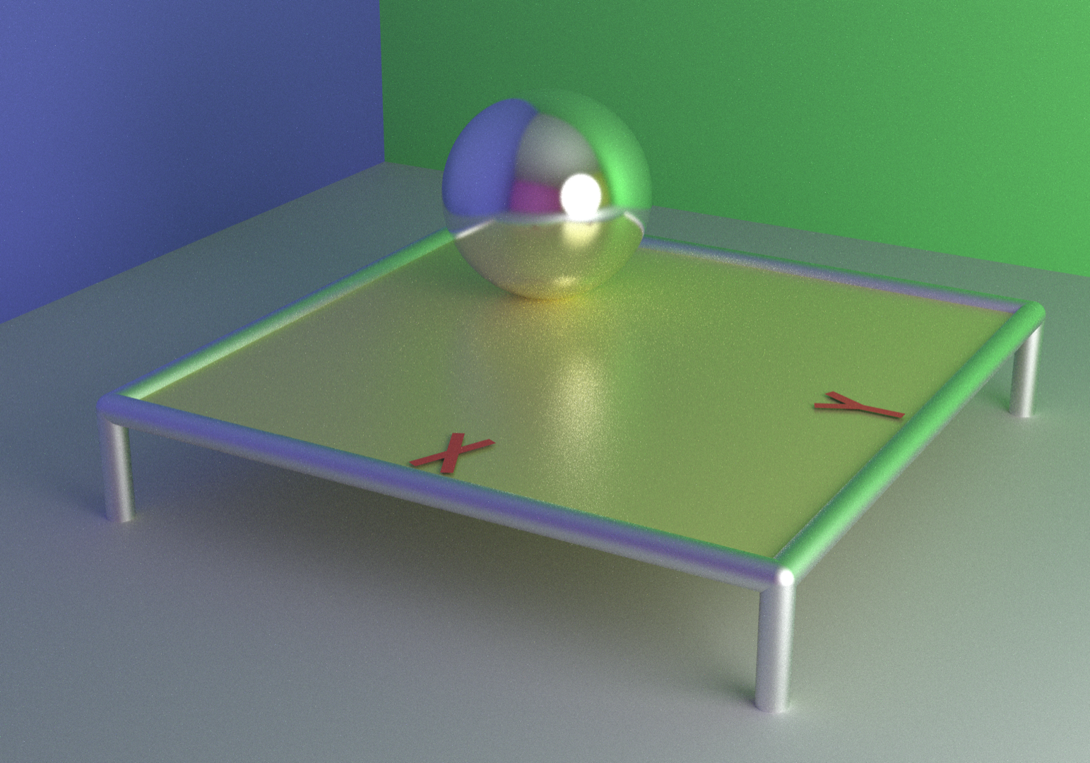
A 256-pass render with equal 0.5f weights: the reflective sphere and its image on the table-top are spotted with bright fireflies. Doubling the samples (below) thins them but doesn’t erase the underlying strategy mismatch.
The fix is to make the weight depend on which strategy was more appropriate at the sampled direction. Multiple Importance Sampling formalizes this: when both strategies could have produced a given direction, weight each in inverse proportion to its probability of having done so. The balance heuristic uses the two PDFs directly:
// Explicit shadow ray contribution
float p_brdf = pdfBrdf(N, inDir, outDir, mat);
float weight = p_light / (p_light + p_brdf);
C += weight * W * (f / p_light) * lightRadiance;

// Implicit BRDF-sampled ray that happened to hit the light
float weight = p_brdf / (p_brdf + p_light);
C += W * weight * lightRadiance;
When a BRDF-sampled ray reaches the light from a low-probability direction (p_brdf small, p_light large), the larger denominator p_brdf + p_light brings the weight down toward zero. The firefly’s contribution collapses, because the explicit strategy could have sampled the same direction much more reliably and contributed the energy without the spike. On purely diffuse surfaces the two PDFs are comparable, the heuristic recovers weights near 0.5f, and the result matches the previous chapter’s behavior.

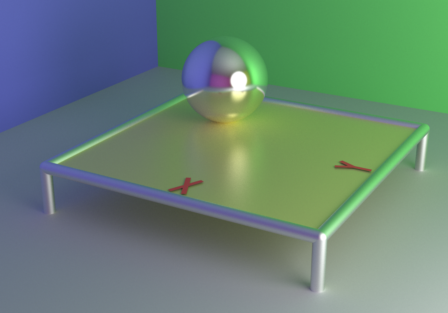
The same scene, same pass count, with the balance heuristic in place. The bulk of the fireflies collapse; a thinner residue survives. The heuristic suppresses low-PDF contributions but doesn’t fully extinguish them. The highlight resolves sharply and the sphere’s reflection reads cleanly across most of the image.
Doubled to 512 passes and placed side by side, the equal-weight render still carries dense firefly residue around the reflective sphere. Variance reduction alone can’t fix a strategy that occasionally emits enormous f / p values. The balance heuristic in the right column collapses the bulk of it, leaving a thinner layer of survivors that no further passes will fully clear:

MIS changes the sampling strategy; it does not clean up the output of a bad one. Sample count cannot substitute for the right strategy. The survivors in the balance-heuristic column show the floor of what this fix can reach: the variance the heuristic itself cannot suppress, no matter how many more passes are spent on it.
A scene that uses what the BRDF can do
With the microfacet BRDF and MIS in place, scenes that earlier rendered as Cornell-box exercises can show off real material variety. A reflective tabletop, a metallic sphere at its center, colored walls bouncing tinted indirect light, fine specular reflections on the floor and on the sphere’s surface.
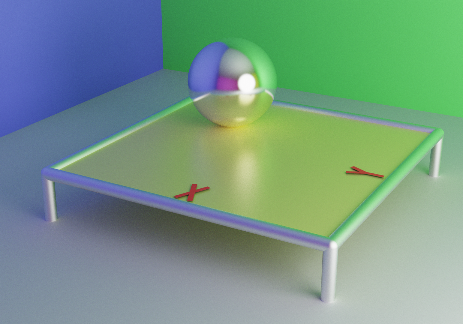
A high-quality render of the baseline scene: the reflective table, the sphere, and the colored walls. The metallic edges of the table pick up the green and blue tints from the surrounding walls. The sphere reflects the overhead light as a sharp highlight and the colored room across its curved surface.
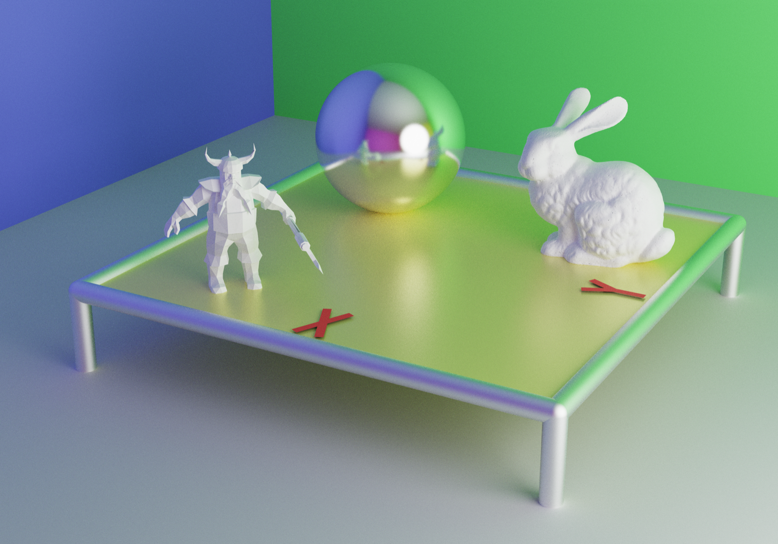
The same setup with two diffuse mesh objects added — a Stanford rabbit and a dwarf — sitting on the reflective table. The diffuse meshes accumulate soft colored bounce light from the walls. The sphere’s reflection picks them up with significant angular distortion (the rabbit’s silhouette is recognizable in the curve), and faint specular reflections of both meshes appear on the table-top.
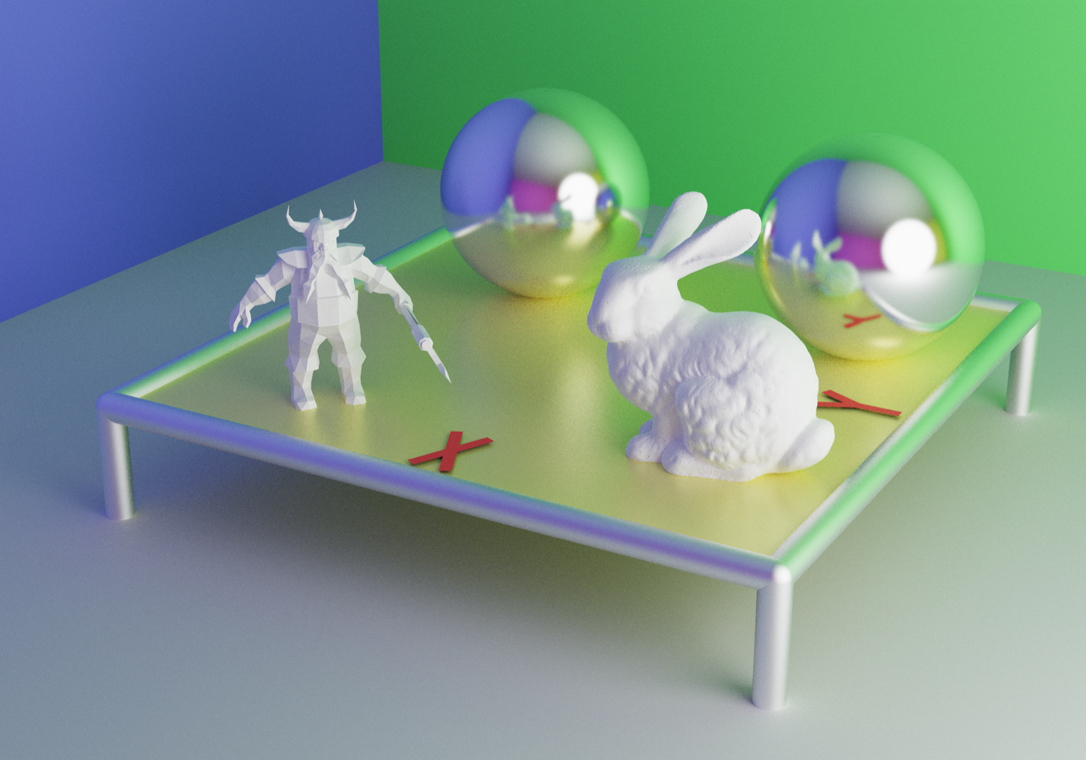
The most demanding configuration: two reflective spheres flanking the diffuse meshes. Each sphere reflects the other and the meshes, producing a network of multi-bounce specular paths. A close inspection of the first sphere reveals the second sphere reflected within it, and within that reflection, a smaller specular highlight nested again: a recursive specular-to-specular path resolved across multiple bounces.
What still cannot pass through
The renderer can now distinguish a metal from a wall, a polished surface from a rough one, a mirror from a piece of paper. But every surface in this chapter still treats every ray the same way: either reflected off the surface or absorbed into it. There is no path that enters a material and continues through it. Glass, water, and tinted plastics can’t be rendered yet because the BRDF stops at the surface, and there is no BTDF (bidirectional transmittance distribution function) to take over from there.
That is the next addition. Snell’s law, total internal reflection, Beer’s law absorption, and the bookkeeping of two indices of refraction are what the next chapter is about. The framework — EvalScattering, pdfBrdf, SampleBRDF — is already abstract enough to absorb a third sampling lobe alongside diffuse and specular reflection. The material system needs to learn about transmission.